1. Purpose

This policy establishes guidelines for the impairment assessment of startup equity investments held by TANAAKK, ensuring compliance with IFRS 9 (Financial Instruments) and IAS 36 (Impairment of Assets).

2. Scope

2.1 Scope

This policy applies to all startup equity investments classified as:

• Financial assets measured at fair value through profit or loss (FVTPL)
• Financial assets measured at fair value through other comprehensive income (FVOCI)
• Equity-accounted investments (IFRS 28 – Associates & Joint Ventures)

2.2 Fair Market Value definition

For income tax purposes, the appropriate standard of value is fair market value (“FMV”), which is defined as

The price, expressed in terms of cash equivalents, at which such property would change hands between a hypothetical willing and able buyer and a hypothetical willing and able seller, acting at arm’s length in an open and unrestricted market, when neither is under compulsion to buy or to sell, and when both have reasonable knowledge of relevant facts.

For financial reporting purposes, the appropriate standard of value is fair value (“FV”), which is defined as:

The amount at which an asset (or liability) could be bought (or incurred) or sold (or settled) in a current transaction between willingparties, that is, other than in a forced or liquidation sale.

3. Initial Recognition & Measurement

3.1 Initial Recognition (IFRS 9 – Financial Instruments)

• Startup equities are initially recognized at fair value, plus transaction costs if classified as FVOCI.
• Investments in privately held startups where fair value is not readily available may be recorded at cost as an approximation, subject to periodic revaluation.

3.2 Measurement Models

TANAAKK will decide FMV by weighing % of multiple valuation model.

• Level 1-1 Market approach (Public Market Quoted Price)
  • Guideline (Comparable) public company method
    • The Guideline (or Comparable) Publicly Traded Company Methodology within the Market Approach relies on an analysis of publicly traded companies similar in industry and/or business model to the Company. This methodology uses these guideline companies to develop relevant market multiples and ratios, using metrics such as revenue, earnings before interest and taxes (EBIT), earnings before interest, taxes, depreciation and amortization (EBITDA), net income and/or tangible book value. These multiples and values are then applied to the Company’s corresponding financial metrics.
• Level 1-2 Market approach (Private Comparable Valuation Techniques)
  • Guideline (Comparable) M&A transaction method
    • The Guideline Transactions Methodology of the Market Approach uses prices paid in merger and acquisitions targeting companies similar to the Subject Company. These acquisition values were used in conjunction with the transaction targets’ financials to calculate implied exit multiples. These multiples are then applied to the Company’s corresponding financial data.
  • Subject Company Transaction Method (Prior Transactions Method)
    • This methodology consists of examining prior transactions of the subject Company. According to the AICPA guidelines, recent securities transactions in the Company’s stock should be considered as a relevant input for computing the enterprise valuation.
• Level 2 Income approach
  • Discounted Cash Flow or Internal Valuation Models)
    • This approach focuses on the income-producing capability of a business. TANAAKK review the Company’s historical financials and any forecasts provided by Management. Startups usually reinvest all its earnings back into the Company to fuel revenue. Growth priority weighted instead of increasing operating margins. TANAAKK will review its economies of scale and operating leverage in earnings growth.
• Level 3 Asset approach
  • The asset approach measures the value of an asset by the cost to recreate or replace it with another of like utility. When applied to the valuation of equity interests in businesses, value is based on the net aggregate fair market value of the entity’s underlying individual assets. This approach is frequently used in valuing holding companies or capital-intensive businesses. This methodology was considered and not used, as it does not accurately represent the going concern value of the Company.
• Others COST TO RECREATE METHOD
  • This method defines an enterprise’s fair market value as the sum total of the enterprise’s assets minus the sum total of the corresponding liabilities. In the case that an enterprise’s assets are not sufficiently captured on its balance sheet, the cost to recreate method assumes that the enterprise’s fair market value is consistent with the replacement cost (i.e. cost to recreate) of the enterprise’s assets.

4. Impairment Testing (IAS 36 – Impairment of Assets)

Impairment is assessed at least annually or when impairment indicators exist.

4.1 Impairment Indicators

• Decline in startup’s market value (if publicly traded).
• Deteriorating financial health, including consistent losses or failure to secure funding.
• Regulatory or legal issues affecting the startup’s viability.
• Failure to meet key business milestones (e.g., product development delays, revenue decline).
• Bankruptcy or liquidation risk.

4.2 Impairment Calculation

1. Fair Value Assessment: Compare the carrying amount to the recoverable amount.
2. Recoverable Amount = Higher of:
   • Fair Value less Costs to Sell (based on recent transactions, funding rounds, or M&A activity)
   • Value in Use (Discounted Cash Flow method for private startups)
3. If Recoverable Amount < Carrying Value, impairment is recorded.
4. Impairment losses for FVTPL equities are recorded in the income statement.
5. Impairment losses for FVOCI equities are recorded in other comprehensive income (OCI) and are not reversed.

5. Special Considerations for Early-Stage Startups

5.1 Investments at Cost (IFRS 9 – Measurement Exception)

• If fair value cannot be reliably measured, investments may be held at cost.
• Annual reassessment required to determine if cost remains a valid approximation of fair value.

5.2 Convertible Instruments & SAFEs (Simple Agreements for Future Equity)

• Assessed for impairment based on:
  • Probability of conversion into equity
  • Risk of total write-off if startup fails
  • Latest funding round valuations

5.3 Option pricing model

• Option pricing model (OPM)
  • The OPM allocates a company’s equity value among the various capital investors. The OPM takes into account the preferred shareholders’ liquidation preferences, participation rights, dividend policy, and conversion rights to determine how proceeds from a liquidity event shall be distributed among the various ownership classes at a future date.
• Probability weighted expected return method (PWERM)
  • The Probability Weighted Expected Return Method of allocating value between security holders analyzes the capital structure of a business at the time of several different potential future outcomes. It assumes that the likelihood, timing, and size of financial success or failure can be estimated. This method involves a forward-looking analysis of the possible future outcomes available to the enterprise, the estimation of ranges of future and present value under each outcome, and the application of a probability factor to each outcome as of the Valuation Date.
• Current value method
  • The Current Value Method allocates the Company’s current value among various equity owners based on liquidation
  • preferences and other rights under the assumption that all capital owners act to maximize their financial
  • return. According to AICPA guidelines, the Current Value Method is applicable in three circumstances: 1) the assumption
  • of an imminent liquidity event in the form of an acquisition or dissolution of a company; 2) when a company
  • is assumed to be at such an early stage of its development that no material progress has been made on its business plan, no significant value has been created above the liquidation preference of the senior securities, and there is no reasonable basis for estimating the amount and timing of any such common equity above the liquidation preference that might be created in the future; and 3) In the case of a simple capital structure, the equity value is allocated pro rata to the common stock, consistent with a Current Value Method allocation methodology.

5.4 Other consideration on premium and discount

• Discount for lack of marketability(DLOM)
  • Both models are commonly used in private company and startup valuations, especially in 409A valuations, shareholder disputes, and tax assessments. The choice between Chaffe and Finnerty depends on the company’s expected liquidity horizon and ability to optimize exit timing.
    • The Chaffe Approach
      • DLOM = Black-Scholes Put Option Value ÷ Stock Price
      • Developed by Chaffe (1993), this approach applies the Black-Scholes Option Pricing Model (BSOPM) to estimate the cost of a put option as a proxy for DLOM. The idea is “A hypothetical shareholder would buy a put option to hedge against the lack of marketability, and the cost of this option represents DLOM.” The cost of a European put option (which can only be exercised at maturity) represents the discount required to compensate for lack of liquidity. DLOM is calculated based on factors such as volatility, time to liquidity, and risk-free rate.The longer the expected holding period, the higher the DLOM, as liquidity is more restricted.
    • The Finnerty Approach
      • DLOM = Lookback Put Option Value ÷ Stock Price
      • Developed by Finnerty (2002), this approach modifies the Chaffe model by using a Lookback Put Option, which allows for greater flexibility in pricing DLOM. A Lookback Put Option gives the holder the right to sell at the highest price observed during the option’s life, better capturing the price fluctuations of non-marketable shares. Produces lower DLOMs than Chaffe’s model, making it more acceptable in some valuation scenarios.
    • Monte Carlo simulation
      • Monte Carlo Simulation is a type of computational algorithm that uses repeated random sampling to obtain the likelihood of a range of results of occurring. John von Neumann and Stanislaw Ulam invented the Monte Carlo simulation, or the Monte Carlo method, in the 1940s. They named it after the famous gambling location in Monaco because the method shares the same random characteristic as a roulette game.
• Weighted Average Cost of Capital (WACC)
  • Capital Asset Pricing Model
    • (“CAPM”) RE = RF + Β * (RM) + SP + CSRP
  • The Capital Asset Pricing Model (CAPM) is used to estimate the cost of equity, which is a key component in discounted cash flow (DCF) valuation and startup valuation models. In general, the higher the WACC, the higher an investor’s expected return would be for an investment in the enterprise.
• SMALL COMPANY SIZE PREMIUM
  • Given that most of the comparable public companies are much larger than the enterprise being valued, there is an additional premium to the cost of equity that investors would requireto invest in small cap public shares.
• COMPANY-SPECIFIC RISK PREMIUM
  • To capture the added risk involved in investing in smaller, less profitable, and less mature companies, an additionalcompany specific risk premium is applied to the cost of equity calculation. This risk premium reflects the additional risk associated with the enterprise’s revenue relative to the market at large.
• COST TO RECREATE METHOD
  • This method defines an enterprise’s fair market value as the sum total of the enterprise’s assets minus the sum total of the corresponding liabilities. In the case that an enterprise’s assets are not sufficiently captured on its balance sheet, the cost to recreate method assumes that the enterprise’s fair market value is consistent with the replacement cost (i.e. cost to recreate) of the enterprise’s assets.

6. Reporting & Disclosure

In accordance with IFRS, the company shall disclose:

1. Significant estimates and judgments used in valuing startup equities.
2. Impairment losses recognized, with a breakdown by investment category.
3. Key assumptions in valuation models for Level 2 & Level 3 investments.
4. Impact of impairment losses on financial statements.

7. Roles & Responsibilities

Role	Responsibility
CFO	Approves impairment assessments and reporting.
Finance Team	Conducts annual and ad-hoc impairment reviews.
Investment Committee	Reviews startup portfolio risk and impairment triggers.
External Auditors	Ensures compliance with IFRS reporting requirements.

8. Policy Review and Updates

This policy shall be reviewed annually to reflect changes in IFRS standards, market conditions, and investment risk factors.

---

Approval & Acknowledgment

Version: v1.1.
Department: Finance & Accounting
Prepared by: Taro Shimizu, Attorney at law Date: 31/12/2024
Approved by: CEO, Shoichiro Tanaka Date: 31/12/2024

---

APPENDIX

STAGE OF DEVELOPMENT

SELECTED STAGE OF DEVELOPMENT: [STAGE XX]

The American Institute of Certified Public Accountants (AICPA) defines six stages of enterprise development:

STAGE ONE

Enterprise has no product revenue to date and limited expense history, and typically an incomplete management team with an idea, plan, and possibly some initial product development. Typically, seed capital or first-round financing is provided during this stage by friends and family, angels, or venture capital firms focusing on earlystage enterprises, and the securities issued to those investors are occasionally in the form of common stock but are more commonly in the form of preferred stock.

STAGE TWO

Enterprise has no product revenue but substantive expense history, as product development is underway and business challenges are thought to be understood. Typically, a second or third round of financing occurs during this stage. Typical investors are venture capital firms, which may provide additional management or board of directors expertise. The typical securities issued to those investors are in the form of preferred stock.

STAGE THREE

Enterprise has made significant progress in product development; key development milestones have been met (for example, hiring of a management team); and development is near completion (for example, alpha and beta testing), but generally there is no product revenue. Typically, later rounds of financing occur during this stage. Typical investors are venture capital firms and strategic business partners. The typical securities issued to those investors are in the form of preferred stock.

STAGE FOUR

Enterprise has met additional key development milestones (for example, first customer orders, first revenue shipments) and has some product revenue, but is still operating at a loss. Typically, mezzanine rounds of financing occur during this stage. Also, it is frequently in this stage that discussions would start with investment banks for an IPO.

STAGE FIVE

Enterprise has product revenue and has recently achieved breakthrough measures of financial success such as operating profitability or breakeven or positive cash flows. A liquidity event of some sort, such as an IPO or a sale of the enterprise, could occur in this stage. The form of securities issued is typically all common stock, with any outstanding preferred converting to common upon an IPO (and perhaps also upon other liquidity events).

STAGE SIX

Enterprise has an established financial history of profitable operations or generation of positive cash flows. An IPO or sale of the enterprise could also occur during this stage.

---

DLOM estimation

Monte Carlo Simulation

1. Parameters for Monte Carlo Simulation

Parameter	Symbol	Definition
Stock Price	S0​ (S_0​)	Initial stock price (e.g., $100)
Expected Return (Drift)	μ(mu)	Expected annual return (e.g., 10%)
Volatility	σ(sigma)	Annual standard deviation of returns (e.g., 40%)
Time Horizon	T	Number of years simulated (e.g., 1 year)
Time Steps	n	Number of intervals in simulation (e.g., 252 trading days)
Risk-Free Rate	r	Annual risk-free rate (e.g., 3%)
Random Shock	Z	Standard normal variable (random number)

2. Monte Carlo Simulation Formula

The Monte Carlo simulation follows the Geometric Brownian Motion (GBM) model, which is based on the Black-Scholes framework:

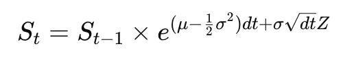
S_t​=S_{t−1}​*e^[{μ−1/2​*(σ^2)}dt+σ√ (dt​Z)]

Where:

• S_t​ = Stock price at time t
• S_{t-1} = Stock price at previous step
• e=Euler’s mathematical constant number (~2.718). It is the base of the natural logarithm (and is widely used in exponential growth models, finance, and probability theory.
• e^(μ−21​σ2)dt = Drift term (expected return adjusted for volatility)
• σ√ (dt​Z) = Random shock (volatility times a random normal variable). Random shocks do not have a fixed constant value—they are generated dynamically in each simulation run using a random number generator (RNG).
• dt=T/n= Time step size (fraction of the year)

3. Monte Carlo Simulation Process

1. Set initial stock price S0​.
2. Define number of simulations (e.g., 1,000 stock price paths).
3. Divide time horizon into small time steps (e.g., 252 for daily trading days).
4. Generate random normal shocks Z.
5. Apply the stock price formula iteratively over the time horizon.
6. Analyze the distribution of final prices to estimate expected return, risk, and DLOM.

4. Key Insights from Monte Carlo for DLOM

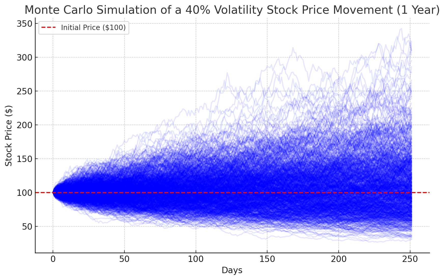
• Higher volatility (σ) → Greater price dispersion → Higher DLOM.
• Longer illiquidity periods (T) → Higher expected discount.
• Simulations can predict probability bands (e.g., 95% confidence interval for price movements).

5. European put option

The Black-Scholes formula for a European put option is:

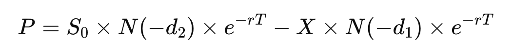
Where:

• P = Price of the put option (cost of marketability restriction)
• S0​ = Current stock price
• X = Strike price (assumed to be equal to S0S_0S0​)
• T = Holding period (in years, typically 2 to 5 years for startups)
• r = Risk-free rate (e.g., 1% – 5%)
• σ = Volatility (typically 40% – 80% for startups)
• N(d) = Cumulative normal distribution function

• Step-by-Step Breakdown:
  • The exact calculation for determining 21.78% DLOM using the Chaffe Approach (Black-Scholes European Put Option Model) is as follows:
• Inputs:
  • Stock price (S) = $100
  • Strike price (K) = $100
  • Risk-free rate (r) = 3% (0.03)
  • Time to liquidity (T) = 1 year
  • Volatility (σ) = 60% (0.6)
• Calculate Intermediate Values:
  • d1=0.35
  • d2=−0.25

6.Typical Percentage Range for Put Option Cost (DLOM Estimate)

The cost of the European put option, representing DLOM, varies based on input assumptions:

Volatility (σ)	Holding Period (T)	DLOM (Put Cost as % of Stock Price)
40%	1 Year	10% – 15%
40%	3 Years	20% – 30%
40%	5 Years	30% – 40%
60%	1 Year	15% – 20%
60%	3 Years	30% – 40%
60%	5 Years	40% – 50%
80%	1 Year	20% – 25%
80%	3 Years	35% – 50%
80%	5 Years	50% – 60%

• For early-stage startups (high volatility, long illiquidity period) → DLOM is often 40% – 60%.
• For later-stage startups (lower volatility, shorter illiquidity period) → DLOM is 20% – 40%.

What d1​ and d2​ mean?

e.g. d1=0.35

• Measures how much the stock price has to move for the option to be in-the-money at expiration.
• Higher d1​ means the option has a higher probability of being exercised.
• d1=0.35 implies about a 63.7% probability (from normal distribution tables) that the stock will finish above the strike price at expiration.

e.g. d2=−0.25

• Accounts for the probability-adjusted discounting of the option’s value.
• It is always lower than d1​ due to the presence of volatility and time decay.
• d2=−0.25 implies about a 40.2% probability that the put option will be in the money at expiration.

Meaning of “In the Money” for a Put Option

Stock Price at Expiration (S_T)
Strike Price (K)

• If S_T < K → The put option is “in the money”(ITM) and has intrinsic value.
• If S_T = K → The put option is “at the money” (ATM) and has no intrinsic value.
• If S_T ​>K → The put option is “out of the money” (OTM) and expires worthless.

7. Example use of Valuation Models

Different valuation models produce different DLOM estimates:

Method	DLOM Range for Early-Stage Startups
Chaffe Approach (BSOPM)	45% – 60%
Finnerty Approach (Lookback Option)	30% – 50%
Restricted Stock Studies	35% – 55%
Pre-IPO Transaction Studies	20% – 40%

8. DLOM Ranges by Startup Stage

Startup Stage	Typical DLOM Range
Pre-Seed / Seed	50% – 60%
Series A	40% – 50%
Series B & Growth	30% – 40%
Pre-IPO	20% – 30%

9. Investors expectation / actual startup equity costs

Capital Asset Pricing Model(CAPM)

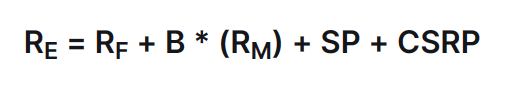
• Re = Return on equity
• Rf = Risk-free rate
• β = Beta
• Rm = Market risk premium
• SP = Small company size premium
• CSRP = Company-specific risk premium

Defining Each Component in Startup Valuation

Risk-Free Rate (rf​)

• Represents a risk-free investment (usually the 10-year US Treasury yield).
• Example: If the 10-year US Treasury rate = 4%, then rf=4%.

Beta (β) – Market Risk Factor

• Measures correlation with the overall market (public stocks).
• Since startups don’t have a public beta, we use industry betas (adjusted for private firms).
• Example: A SaaS startup might have β=1.8 (higher than the market average of 1.0).

Equity Risk Premium (rm​−rf​)

• The expected return above risk-free investments (historically 5% – 7% in the US).
• Example: If market return = 9% and rf=4%, then: ERP=rm−rf=9%−4%=5%

Small Size Premium (SSP)

• Small companies are riskier than large public firms.
• Empirical studies show SSP = 2% – 6% for private startups.
• Example: If a startup is early-stage, SSP = 4%.

Company-Specific Risk Premium (CSRP)

• Extra premium for startup-specific risks, like:
  • No revenue/profit history
  • Market uncertainty
  • Regulatory risks
• Typically CSRP = 5% – 15% based on startup risk profile.
• Example: A biotech startup with high uncertainty might have CSRP = 10%.

Assume a startup has the following parameters:

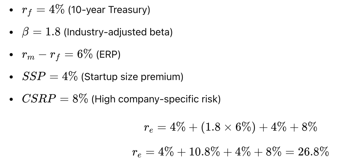
Estimated cost of equity = 26.8%

This means investors expect at least 26.8% annual return to compensate for the startup’s risk.

---

About constant number “e”

Euler’s number arises in situations involving continuous growth. The most common interpretation is in compound interest and natural exponential growth.

Definition of e

Euler’s number is defined as:

e=lim⁡_{n→∞}(1+1/n)^n

This formula shows that as n increases indefinitely, the expression approaches 2.718.

2. Why Is e Important?

e appears in many real-world applications:

1. Continuous Compound Interest

If you invest $1 at an interest rate r for t years, with continuous compounding, the value grows

A=Pe^rt

where:

• P = Principal amount
• r = Interest rate
• t = Time in years

Example: At 100% annual interest (r=1), your money grows to e≈2.718 (approx) after 1 year.

2. Exponential Growth & Decay

Many natural phenomena follow an exponential function using e:

• Population Growth: N(t) = N_0 e^{rt}
• Radioactive Decay: N(t)=N_0 e^{-kt}
• Cooling of Objects (Newton’s Law of Cooling)

3. Probability & Statistics (Poisson Process)

• Used in modeling random events over time, such as:
  • Number of emails received per hour
  • Stock price fluctuations
  • Queuing theory in traffic & server loads